Risk Management Study Guide

In-Person: NY Wall Street
Campus
Duration : 5 Days (Full-time)
Teaching Mode : Live Instructor Classes


Virtual Live
Duration : 5 Days
Teaching Mode : Live Virtual Sessions


Self-Paced Online
Duration : 40 Hours (Learn at your pace)
Teaching Mode : Recorded Sessions +
Q&A with Faculty


Imagine a financial institution navigating a sudden market downturn. The firm faces multiple risks, including market, credit, and operational risks. The management's ability to quickly identify, assess, and mitigate these risks determines whether the firm will survive or suffer significant losses.
Protect assets, ensure business stability, and maintain compliance with regulations. In the example above, managing these risks effectively prevented catastrophic losses and ensured continued operations.
Market Risk : Fluctuations in stock prices and interest rates.
Credit Risk : Potential default by borrowers.
Operational Risk : Failures in internal processes or systems.


Market and Credit Risk Interaction : In a financial crisis, a drop in market value can lead to credit downgrades, increasing the likelihood of defaults and exacerbating credit risk.

During the 2008 financial crisis, falling real estate prices (market risk) led to widespread mortgage defaults (credit risk), causing significant losses for financial institutions.

Cognitive Biases : Overconfidence, loss aversion, and herd behavior can exacerbate financial risks. For example, overconfidence can lead to underestimating risks, while herd behavior can drive market bubbles and crashes.
This means there is a 5% chance that the portfolio could lose 26% or more over the next 10 days.
VaR = 1.6 × 0.05 × 10 = 0.26

Example : For a portfolio with a standard deviation of 5%, a time horizon of 10 days, and a 95% confidence level (Z-Score = 1.65), the VaR would be:
VaR = Z-Score × σ ×


EL = 0.02 × 1,000,000 × 0.60 = 12,000
Example : If a loan has a 2% PD, an EAD of $1 million, and an LGD of 60%, the expected loss would be:
PD: Probability of Default.
EAD: Exposure at Default.
LGD: Loss Given Default.
EL = PD × EAD × LGD


Equity Risk Management: A portfolio manager anticipates a market downturn and uses options to hedge against potential losses. By buying put options, the manager can limit downside risk while retaining upside potential.
Example : For an asset with a beta of 1.2, a risk-free rate of 2%, and a market return of 8%, the expected return would be:
Capital Asset Pricing Model (CAPM):
Expected Return = Rf +β(Rm− Rf)
Expected Return = 0.02 + 1.2 × (0.08 − 0.02) = 0.092 = 9.2%
Market Line


World
Index
Investable
Assets


/ (1 + y)

Example : For a bond with cash flows of $100 annually, a yield of 5%, and a current price of $950, the duration measures the bond's sensitivity to interest rate changes.

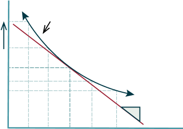
Increaseing price
sensitivity to yeield changes

Decreasing price
sensitivity to yeield changes


Advanced Risk Metrics and Models

Value at Risk (VaR) : Used daily by trading desks to estimate potential losses. However, during extreme market conditions, VaR may underestimate risk, as seen in the 2008 crisis when actual losses exceeded VaR estimates.
ES = E [ L | L > VaR ]
Example : If the VaR is $1 million, and the average loss beyond this threshold is $1.5 million, the ES would be $1.5 million, providing a more comprehensive risk assessment.


Advanced Risk Metrics and Models

Explanation : This ratio helps validate the accuracy of VaR models by comparing observed losses with expected outcomes.


exceedances


Derivatives, Futures, Swaps, and Options

Example : For a swap with a notional value of $1 million, a fixed rate of 3%, and a floating rate of SOFR + 1%, the NPV calculation involves determining the sum of the differences between the present values of the fixed and floating payments for each period in the swap.
Fixed Rate / Floating Rate : Agreed fixed or variable rate.
Notional : Principal amount for interest calculations.
y(t) : Discount rate for each period t.
( Fixed Rate × Notional )

( Floating Rate × Notional )


The Black-Scholes model is used to price European options. While critical, the full formula is complex, so users are directed to more detailed resources for a complete understanding.
Note on Black-Scholes Formula :


Variables


Types


Models
Pricing

Basel III requires banks to maintain higher capital reserves—funds set aside to absorb losses—impacting how much they can lend. This regulation also imposes stricter operational controls, such as closer monitoring of capital levels and more frequent reporting to regulators.

The Dodd-Frank Act introduces significant challenges for financial institutions, particularly in derivatives trading, where banks must manage contracts that derive value from underlying assets. The Volcker Rule, a key component of Dodd-Frank, restricts proprietary trading—trading for the bank's own profit. This requires banks to overhaul their trading strategies and implement systems to ensure compliance, leading to increased operational complexity and costs.

Focuses on ensuring that banks have adequate capital to absorb losses (capital adequacy), conducting stress tests to simulate extreme economic conditions, and maintaining market liquidity—the ability to quickly convert assets into cash.

Aims to reduce systemic risk—the risk that the failure of one institution could lead to a broader financial collapse—by imposing tighter regulations on financial institutions.


Capital Reserve Requirements
Before basel lll
Capital Reserve Requirements
After basel lll


Banks use AI models to assess borrower creditworthiness, analyzing vast amounts of data to predict defaults more accurately than traditional models.
AI in Credit Risk :

Investment firms analyze large datasets to identify emerging risks, such as sector-specific vulnerabilities during economic downturns.

Automates risk identification and assessment processes.


Enhances predictive accuracy in risk modeling.

& Case Studies

COVID-19 Pandemic : Financial institutions used stress testing and scenario analysis to navigate unprecedented market volatility. These tools helped them adjust risk management strategies in real-time, demonstrating the importance of flexible frameworks.
Cybersecurity Risk : A large financial institution faced a major cyberattack, prompting an overhaul of its operational risk management practices. This case illustrates the growing importance of integrating cybersecurity into risk management.
Liquidity-Adjusted VaR : During the 2008 financial crisis, traditional VaR models underestimated risk due to the lack of liquidity adjustment. Incorporating liquidity risk into VaR models provides a more accurate picture of potential losses during market stress.

Risk Management Study Guide

Duration : 5 Days (Full-time)
Teaching Mode : Live Instructor Classes


Teaching Mode : Live Virtual Sessions

Duration : 40 Hours (Learn at your pace)
Teaching Mode : Recorded Sessions +


Imagine a financial institution navigating a sudden market downturn. The firm faces multiple risks, including market, credit, and operational risks. The management's ability to quickly identify, assess, and mitigate these risks determines whether the firm will survive or suffer significant losses.
Protect assets, ensure business stability, and maintain compliance with regulations. In the example above, managing these risks effectively prevented catastrophic losses and ensured continued operations.
Market Risk : Fluctuations in stock prices and interest rates.
Credit Risk : Potential default by borrowers.
Operational Risk : Failures in internal processes or systems.


Market and Credit Risk Interaction : In a financial crisis, a drop in market value can lead to credit downgrades, increasing the likelihood of defaults and exacerbating credit risk.

During the 2008 financial crisis, falling real estate prices (market risk) led to widespread mortgage defaults (credit risk), causing significant losses for financial institutions.

Cognitive Biases : Overconfidence, loss aversion, and herd behavior can exacerbate financial risks. For example, overconfidence can lead to underestimating risks, while herd behavior can drive market bubbles and crashes.
This means there is a 5% chance that the portfolio could lose 26% or more over the next 10 days.
VaR = 1.6 × 0.05 × 10 = 0.26

Example : For a portfolio with a standard deviation of 5%, a time horizon of 10 days, and a 95% confidence level (Z-Score = 1.65), the VaR would be:
VaR = Z-Score × σ ×


EL = 0.02 × 1,000,000 × 0.60 = 12,000
Example : If a loan has a 2% PD, an EAD of $1 million, and an LGD of 60%, the expected loss would be:
PD: Probability of Default.
EAD: Exposure at Default.
LGD: Loss Given Default.
EL = PD × EAD × LGD


Equity Risk Management: A portfolio manager anticipates a market downturn and uses options to hedge against potential losses. By buying put options, the manager can limit downside risk while retaining upside potential.
Example : For an asset with a beta of 1.2, a risk-free rate of 2%, and a market return of 8%, the expected return would be:
Capital Asset Pricing Model (CAPM):
Expected Return = Rf +β(Rm− Rf)
Expected Return = 0.02 + 1.2 × (0.08 − 0.02) = 0.092 = 9.2%
Market Line


World
Index
Investable
Assets


/ (1 + y)

Example : For a bond with cash flows of $100 annually, a yield of 5%, and a current price of $950, the duration measures the bond's sensitivity to interest rate changes.

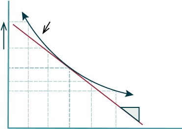
Increaseing price
sensitivity to yeield changes

Decreasing price
sensitivity to yeield changes


Advanced Risk Metrics and Models

Value at Risk (VaR) : Used daily by trading desks to estimate potential losses. However, during extreme market conditions, VaR may underestimate risk, as seen in the 2008 crisis when actual losses exceeded VaR estimates.
ES = E [ L | L > VaR ]
Example : If the VaR is $1 million, and the average loss beyond this threshold is $1.5 million, the ES would be $1.5 million, providing a more comprehensive risk assessment.


Explanation : This ratio helps validate the accuracy of VaR models by comparing observed losses with expected outcomes.


exceedances


Example : For a swap with a notional value of $1 million, a fixed rate of 3%, and a floating rate of SOFR + 1%, the NPV calculation involves determining the sum of the differences between the present values of the fixed and floating payments for each period in the swap.
Fixed Rate / Floating Rate : Agreed fixed or variable rate.
Notional : Principal amount for interest calculations.
y(t) : Discount rate for each period t.
( Fixed Rate × Notional )

( Floating Rate × Notional )


The Black-Scholes model is used to price European options. While critical, the full formula is complex, so users are directed to more detailed resources for a complete understanding.
Note on Black-Scholes Formula :


Variables


Types


Models
Pricing

Basel III requires banks to maintain higher capital reserves—funds set aside to absorb losses—impacting how much they can lend. This regulation also imposes stricter operational controls, such as closer monitoring of capital levels and more frequent reporting to regulators.

The Dodd-Frank Act introduces significant challenges for financial institutions, particularly in derivatives trading, where banks must manage contracts that derive value from underlying assets. The Volcker Rule, a key component of Dodd-Frank, restricts proprietary trading—trading for the bank's own profit. This requires banks to overhaul their trading strategies and implement systems to ensure compliance, leading to increased operational complexity and costs.

Focuses on ensuring that banks have adequate capital to absorb losses (capital adequacy), conducting stress tests to simulate extreme economic conditions, and maintaining market liquidity—the ability to quickly convert assets into cash.

Aims to reduce systemic risk—the risk that the failure of one institution could lead to a broader financial collapse—by imposing tighter regulations on financial institutions.


Capital Reserve Requirements
Before basel lll
Capital Reserve Requirements
After basel lll
Integration of Technology in
Risk Management

Banks use AI models to assess borrower creditworthiness, analyzing vast amounts of data to predict defaults more accurately than traditional models.
AI in Credit Risk :

Investment firms analyze large datasets to identify emerging risks, such as sector-specific vulnerabilities during economic downturns.

Automates risk identification and assessment processes.


Enhances predictive accuracy in risk modeling.
& Case Studies

COVID-19 Pandemic : Financial institutions used stress testing and scenario analysis to navigate unprecedented market volatility. These tools helped them adjust risk management strategies in real-time, demonstrating the importance of flexible frameworks.
Cybersecurity Risk : A large financial institution faced a major cyberattack, prompting an overhaul of its operational risk management practices. This case illustrates the growing importance of integrating cybersecurity into risk management.
Liquidity-Adjusted VaR : During the 2008 financial crisis, traditional VaR models underestimated risk due to the lack of liquidity adjustment. Incorporating liquidity risk into VaR models provides a more accurate picture of potential losses during market stress.
© 2023 NYIF.com. All Right Reserved. NYIF is licensed by the New York State Education Department (NYSED) and registered with the National Association of State Boards of Accountancy (NASBA).

Risk Management Study Guide

In-Person: NY Wall Street
Campus
Duration : 5 Days (Full-time)
Teaching Mode : Live Instructor Classes


Virtual Live
Duration : 5 Days
Teaching Mode : Live Virtual Sessions


Self-Paced Online
Duration : 40 Hours (Learn at your pace)
Teaching Mode : Recorded Sessions +
Q&A with Faculty


Imagine a financial institution navigating a sudden market downturn. The firm faces multiple risks, including market, credit, and operational risks. The management's ability to quickly identify, assess, and mitigate these risks determines whether the firm will survive or suffer significant losses.
Protect assets, ensure business stability, and maintain compliance with regulations. In the example above, managing these risks effectively prevented catastrophic losses and ensured continued operations.
Market Risk : Fluctuations in stock prices and interest rates.
Credit Risk : Potential default by borrowers.
Operational Risk : Failures in internal processes or systems.


Market and Credit Risk Interaction : In a financial crisis, a drop in market value can lead to credit downgrades, increasing the likelihood of defaults and exacerbating credit risk.

During the 2008 financial crisis, falling real estate prices (market risk) led to widespread mortgage defaults (credit risk), causing significant losses for financial institutions.

Cognitive Biases : Overconfidence, loss aversion, and herd behavior can exacerbate financial risks. For example, overconfidence can lead to underestimating risks, while herd behavior can drive market bubbles and crashes.
This means there is a 5% chance that the portfolio could lose 26% or more over the next 10 days.
VaR = 1.6 × 0.05 × 10 = 0.26

Example : For a portfolio with a standard deviation of 5%, a time horizon of 10 days, and a 95% confidence level (Z-Score = 1.65), the VaR would be:
VaR = Z-Score × σ ×

PD: Probability of Default.
EAD: Exposure at Default.
LGD: Loss Given Default.
Example : If a loan has a 2% PD, an EAD of $1 million, and an LGD of 60%, the expected loss would be:
EL = PD × EAD × LGD
EL = 0.02 × 1,000,000 × 0.60 = 12,000


Equity Risk Management: A portfolio manager anticipates a market downturn and uses options to hedge against potential losses. By buying put options, the manager can limit downside risk while retaining upside potential.
Example : For an asset with a beta of 1.2, a risk-free rate of 2%, and a market return of 8%, the expected return would be:
Capital Asset Pricing Model (CAPM):
Expected Return = Rf +β(Rm− Rf)
Expected Return = 0.02 + 1.2 × (0.08 − 0.02) = 0.092 = 9.2%
Market Line


World
Index

Investable
Assets


/ (1 + y)

Example : For a bond with cash flows of $100 annually, a yield of 5%, and a current price of $950, the duration measures the bond's sensitivity to interest rate changes.


Increaseing price
sensitivity to yeield changes
Decreasing price
sensitivity to yeield changes


Advanced Risk Metrics and Models

Value at Risk (VaR) : Used daily by trading desks to estimate potential losses. However, during extreme market conditions, VaR may underestimate risk, as seen in the 2008 crisis when actual losses exceeded VaR estimates.
ES = E [ L | L > VaR ]
Example : If the VaR is $1 million, and the average loss beyond this threshold is $1.5 million, the ES would be $1.5 million, providing a more comprehensive risk assessment.


Explanation : This ratio helps validate the accuracy of VaR models by comparing observed losses with expected outcomes.


exceedances


Example : For a swap with a notional value of $1 million, a fixed rate of 3%, and a floating rate of SOFR + 1%, the NPV calculation involves determining the sum of the differences between the present values of the fixed and floating payments for each period in the swap.
Fixed Rate / Floating Rate : Agreed fixed or variable rate.
Notional : Principal amount for interest calculations.
y(t) : Discount rate for each period t.
( Fixed Rate × Notional )

( Floating Rate × Notional )


Variables


Types


Models
Pricing
The Black-Scholes model is used to price European options. While critical, the full formula is complex, so users are directed to more detailed resources for a complete understanding.
Note on Black-Scholes Formula :

Basel III requires banks to maintain higher capital reserves—funds set aside to absorb losses—impacting how much they can lend. This regulation also imposes stricter operational controls, such as closer monitoring of capital levels and more frequent reporting to regulators.

The Dodd-Frank Act introduces significant challenges for financial institutions, particularly in derivatives trading, where banks must manage contracts that derive value from underlying assets. The Volcker Rule, a key component of Dodd-Frank, restricts proprietary trading—trading for the bank's own profit. This requires banks to overhaul their trading strategies and implement systems to ensure compliance, leading to increased operational complexity and costs.

Focuses on ensuring that banks have adequate capital to absorb losses (capital adequacy), conducting stress tests to simulate extreme economic conditions, and maintaining market liquidity—the ability to quickly convert assets into cash.

Aims to reduce systemic risk—the risk that the failure of one institution could lead to a broader financial collapse—by imposing tighter regulations on financial institutions.


Capital Reserve Requirements
Before basel lll
Capital Reserve Requirements
After basel lll
Integration of Technology in Risk Management

Banks use AI models to assess borrower creditworthiness, analyzing vast amounts of data to predict defaults more accurately than traditional models.
AI in Credit Risk :

Investment firms analyze large datasets to identify emerging risks, such as sector-specific vulnerabilities during economic downturns.

Risk Management Information Systems (RMIS) :
Automates risk identification and assessment processes.

Enhances predictive accuracy in risk modeling.

Practical Applications & Case Studies
COVID-19 Pandemic : Financial institutions used stress testing and scenario analysis to navigate unprecedented market volatility. These tools helped them adjust risk management strategies in real-time, demonstrating the importance of flexible frameworks.
Cybersecurity Risk : A large financial institution faced a major cyberattack, prompting an overhaul of its operational risk management practices. This case illustrates the growing importance of integrating cybersecurity into risk management.
Liquidity-Adjusted VaR : During the 2008 financial crisis, traditional VaR models underestimated risk due to the lack of liquidity adjustment. Incorporating liquidity risk into VaR models provides a more accurate picture of potential losses during market stress.

